Drawdown

A measure of decline from peak to trough in the value of an investment.

Published

23 January 2025

The drawdown of a series is defined as the decline in value from a pervious peak. More formally, if $Y(t)$ is a stochastic process with $t \geq 0$ and observations $y_t$ , the drawdown at time $t$ is

$\begin{aligned} D(t) = \max_{t^\prime \leq t} \, y_{t^\prime} - y_t, \end{aligned}$

which captures the difference between the highest point reached up to time $t$ and the current value. One may also be concered with the maximum drawdown over the entire history up to time $t$ , given by

$\begin{aligned} \overline{D}(t) = \max_{\tau \leq t} \, D(\tau). \end{aligned}$

Visualizing Drawdown

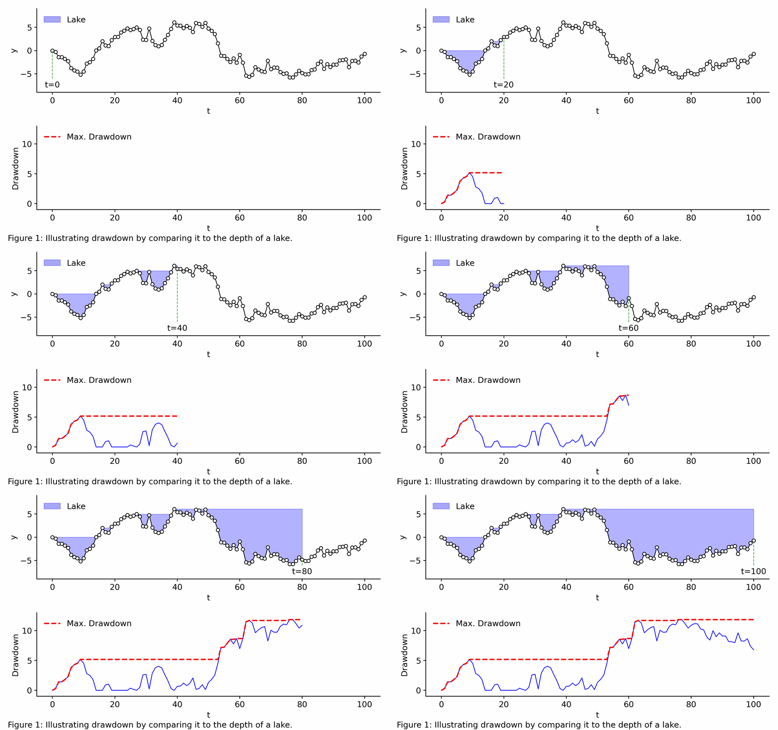
Imagine the time series observed from $Y(t)$ is a landscape that floods whenever its value drops below the highest peak reached so far, creating a lake. Because the data is ordered chronologically, any trough is instantly filled with water from its left edge up to that peak. At any time $t$ , the drawdown is simply the current depth of the lake. The maximum drawdown is simply the deepest point in the lake so far, as shown below.

import numpy as np, matplotlib.pyplot as plt, io
import imageio.v2 as imageio
from tfds.plotting import prettify

plt.rcParams["font.size"] = 12
np.random.seed(9)

xs = np.arange(101)
ys = np.cumsum(np.random.randn(101))

with imageio.get_writer(
    "drawdown.gif", mode="I", duration=150, loop=0
) as writer:
    for i in xs:
        fig, (ax1, ax2) = plt.subplots(2, 1, figsize=(8, 5), sharex=True)
        ax1.plot(xs, ys, "k-o", lw=1, ms=5, mfc="w")
        ax1.fill_between(
            xs[: i + 1],
            ys[: i + 1],
            np.maximum.accumulate(ys[: i + 1]),
            color="b",
            alpha=0.3,
            label="Lake",
        )
        ax1.plot([i, i], [ys.min() - 0.3, ys[i]], "g--", lw=1, alpha=0.7)
        ax1.text(i, ys.min() - 2.2, f"t={i}", ha="center")
        ax1.set(xlabel="t", ylabel="y", ylim=(-9, 9))
        prettify(ax=ax1, legend=True, legend_loc="upper left")

        drawdown = np.maximum.accumulate(ys[: i + 1]) - ys[: i + 1]
        ax2.plot(xs[: i + 1], drawdown, "b-", lw=1)
        ax2.plot(
            xs[: i + 1],
            np.maximum.accumulate(drawdown),
            "r--",
            lw=2,
            label="Max. Drawdown",
        )
        ax2.set(xlabel="t", ylabel="Drawdown", ylim=(-1, 13))
        prettify(ax=ax2, legend=True, legend_loc="upper left")

        fig.text(
            0.02,
            0.01,
            "Figure 1: Illustrating drawdown by comparing it to the depth of a lake.",
            ha="left",
        )
        fig.tight_layout()

        buf = io.BytesIO()
        fig.savefig(buf, format="png", dpi=300)
        plt.close(fig)
        buf.seek(0)
        writer.append_data(imageio.imread(buf))

Application

For investors, a drawdown can be seen as the “pain period” between a peak in returns and the subsequent trough. In short, it’s not just about how high returns can climb, but equally important to understand how far they can drop before they rebound.

Maximum drawdown is often seen as a practical risk indicator because it highlights not just volatility, but the depth of losses an investment might endure. It’s used in various performance metrics, for example the Sterling ratio, which modifies the traditional Sharpe ratio by substituting the standard deviation of returns with some measure of drawdown.